N.B. This was originally a talk at the Weigel Lab, simply copy-pasted to this blog. If you want something actually useful, read the papers linked from here, particularly the review by Ralph & Bradburd, and Wang & Bradburd 2014.

Popgen refresher

• Central idea: subsets of a species are more or less related to other subsets == Population Structure
• Population structure is fractal: from subspecies (e.g. relicts) through continental (Iberia vs W. Europe), regional (Baden-Württemberg vs Hesse), local (Tübingen vs Reutlingen), and hyperlocal (adjacent farms) scales.
• Commonly measure divergence with e.g. $F_{ST}$
• Patterns of divergence among subpopulations can enlighten us as to the processes underlying the evolution of these populations

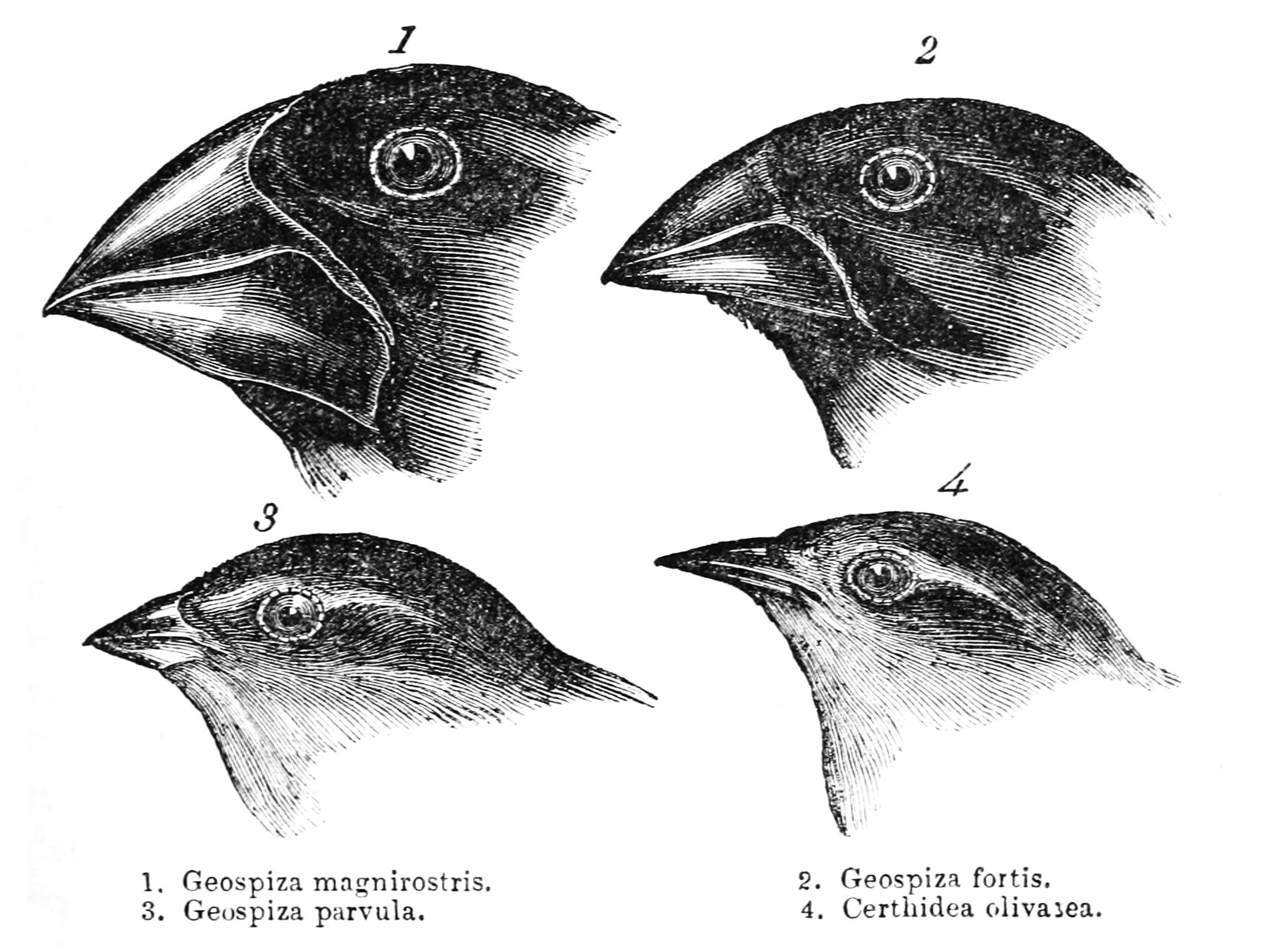
Population genetics is concerned with the observable genetic differences between groups of individuals within some species, and with the historical processes that have lead to these differences. Exceptionally few organisms fit the “null hypothesis” of population genetics: random mating among individuals (panmixia). Four key processes are central to population genetics: Mutations arise, and are then subject to Selection, Drift, Gene flow, which shape the spread (or not) of the mutation through the population, with consequences on the observed frequency of each mutation across the range of the species. Through studying the ways in which the individuals are non-uniformly related, we may gain insights into these processes underlying their evolution.

Population genomics reformulates population genetics in the era of genomics. It applies the theory and models of population genetics, traditionally focused on individual loci, to genome-wide variation among individuals of some species. Through studying multiple loci in each species, we can not only gain insights into the evolution of the individuals that comprise that species, but also the genes that comprise each individual.

Spatial population genetics: patterns of divergence

• Nearly all species have populations and subpopulations which exhibit non-equal relatedness.
• Examining this genome-average relatedness can inform about demography, life history, and gene flow
• Genome-average relatedness needs to be accounted for in future analyses

Few species are panmictic, and the ways in which individuals are related can inform evolutionary hypotheses. In most species, geographically proximate individuals have a far greater chance of interbreeding than individuals separated by a significant distance. Similarly, discrete subpopulations of individuate form through either prolonged geographic separation or ecological differentiation. Either case leads to geographically-structured populations of individuals.

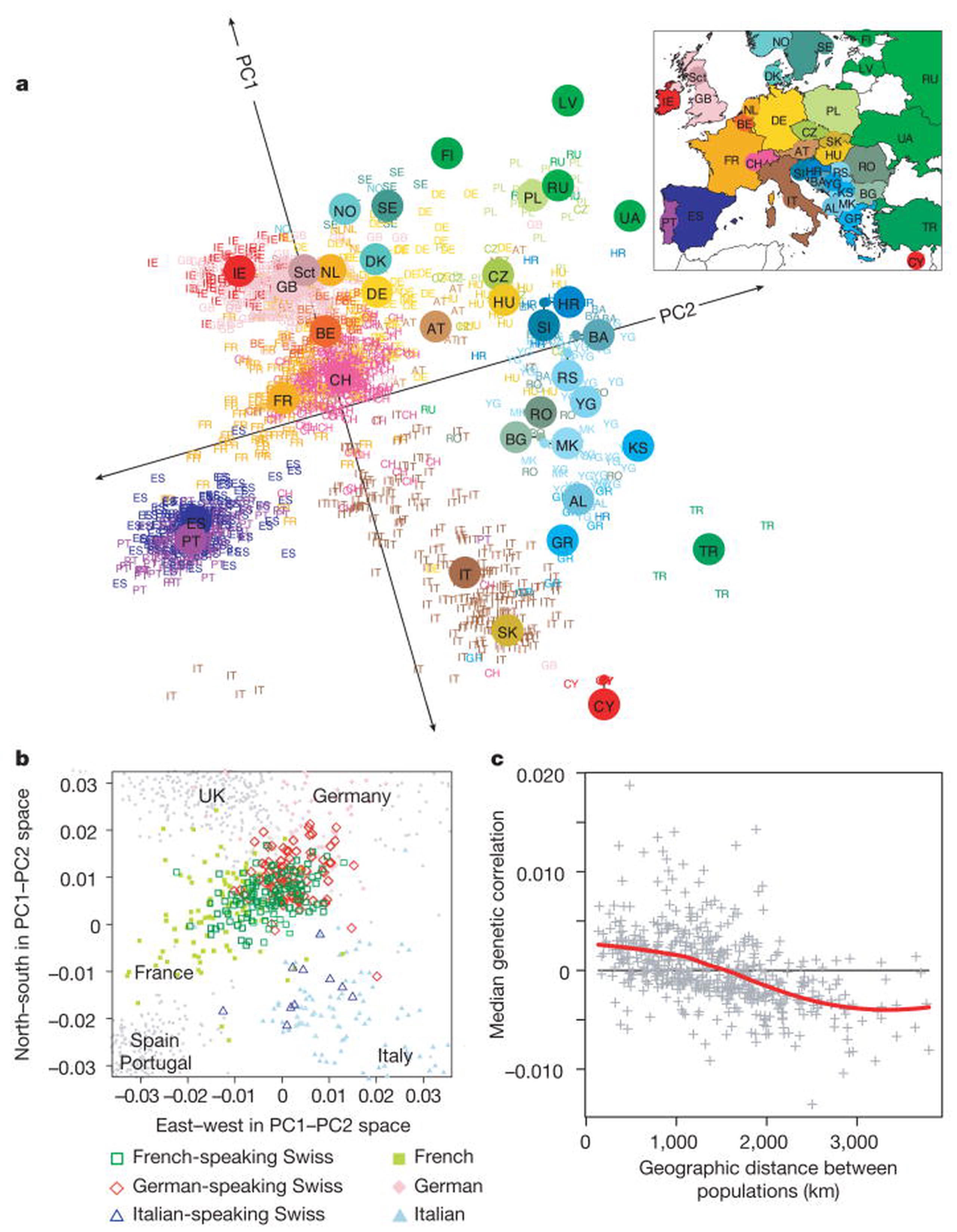
Whereas genetic populations were traditionally modeled as differentiated islands (after Wright), spatial population genetics typically considers each individual or local subpopulation as a geolocated entity within a continuous landscape of individuals. A classic demonstrative example of this is John Novembre’s 2008 paper showing that genetic variation among European humans closely mirrors the geographic location of their recent ancestors.

Reading List

• Bradburd and Ralph, “Spatial Population Genetics: It’s About Time”, Annual Review of Ecology, Evolution, and Systematics (2019)
• Novembre et al., “Genes mirror geography with Europe”, Nature (2008)

An aside: Processes vs patterns

• Two broad styles to approach population genetics/genomics: patterns and processes
• Process-based analyses fit observations to a theoretical model of evolution
• Pattern-based analyses simply describe the form of evolution
• (Opinion) Generally, pattern-based approaches are less easy to over-interpret, and process-based models require more and higher-quality data.

In a well-controlled experiment, we can use relatively simple statistics to conclusively reject null hypotheses, and come as close to proving an effect as is epistemologically possible. We have no such luxury in retrospective studies of evolution. Without access to time-travel, many features of the evolution of populations are fundamentally unknowable or unprovable. As such, we rely on two broad analytic frameworks: fitting data to theoretical models of evolution, or simply describing the current patterns within observed data. As an example, STRUCTURE imposes a model of ancestral populations and recent admixture onto genetic data, whereas PCA simply shows you a low-rank approximation of your data. It is important to keep this distinction in mind when interpreting results: pattern-based approaches imply no particular mechanism, and model-based approaches only imply specific processes if assumptions are met.

Reading list

• Lawson et al., “A tutorial on how not to over-interpret STRUCTURE and ADMIXTURE bar plots”, Nature Comms. 2018
• Wang & Bradburd, “Isolation by Environment”, Molecular Ecology (2014)

Continuous and discrete structure

• Population Structure often considered discrete: modern genetics reflects descendants of and admixture between several ancestral populations.
• Population structure can also be continuous: e.g. Isolation By Distance (IBD) or Isolation by Environment (IBE)
• (Opinion) To me, one should not invoke discrete population structure to explain a continuous pattern of IBD, even at continental scales. Use joint tests (conStruct).

Often, population structure is conceived of as differences between discrete groups, possibly with recent admixture in some individuals/subpopulations. This model both clearly applies at some level, and but is inadequate to describe the geographic structure of individuals across the range of the species. In addition to discrete population structure, within populations the relatedness of individuals typically decays as a function of their geographic distance (Isolation by Distance; IBD). Modern methods and syntheses jointly consider both continuous and discrete patterns of spatial genetic structure.

Importantly, spatial genetic structure of any form is a pattern, and its presence or particular form does not prove the action of any specific evolutionary process. A multitude of both neutral and adaptive processes can generate identical patterns, e.g. a pattern of continuous isolation by distance could be due to mating/migration within a limited range, range expansion, or local adaptation (or many many other causes).

Methods:

• Discrete: PSD model of STRUCTURE & friends: ancestral populations and recent combinations thereof. (STRUCTURE, ADMIXTURE, fastStructure, etc.)
• Continuous: Mantel tests, Generalised Dissimilarity Modelling (see below)
• Join models of Continuous and Discrete structure: recent methods like conStruct

Reading List:

• Bradburd et al., “Inferring Continuous and Discrete Population Genetic Structure Across Space”, Genetics (2017)

Examining Isolation by Distance

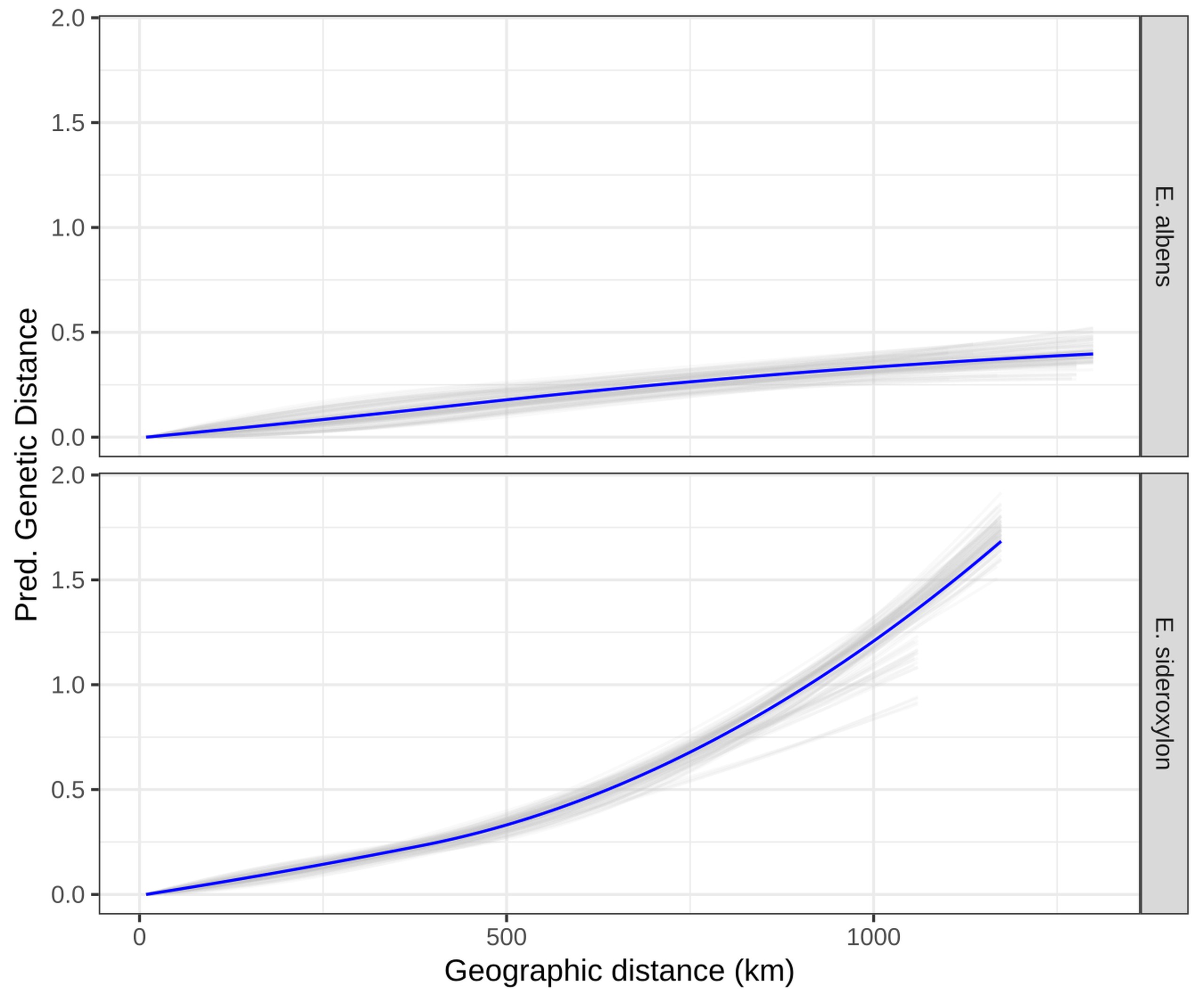
• Isolation by Distance: geographically proximal populations are more closely related than distal populations (i.e. $G \sim D$)
• A pattern, but an informative one with many forms.

Isolation by Distance is a simple statistical pattern whereby average relatedness between individuals decays as a function of their geographic separation. Such a pattern is evident in the vast majority of species, due to limited dispersal of genes (amongst a huge variety of other causes). The precise extent and pattern of Isolation by Distance can be investigated using any number of statistical approaches that probe the correlation between genetic and geographic distances. Mantel tests are a simple permutation-based approach that tests for a linear correlation between genetic distance (e.g. $F_{ST}$ between demes) and geographic distance (e.g. great circle distances between deme locations). Generalised Dissimilarity Modelling is a method that dissects this relationship further, fitting splines to the relationship between genetic and geographic distances.

Methods

• Traditionally, mantel tests were used, but have statistical issues and don’t fully explore pattern
• Nowadays, matrix regression or Generalised Dissimilarity Models (GDMs) provide more statistical rigour and flexibility
• Also, conStruct’s joint discrete/continuous structure models (see above).

Reading List

• Wright, “Isolation by Distance”, Genetics, 1943
• Meirmans, “The trouble with Isolation by Distance”, Molecular Ecology, 2012
• Murray et al., “Landscape drivers of genomic diversity and divergence in woodland Eucalyptus”, Molecular Ecology, 2019

Migration surfaces

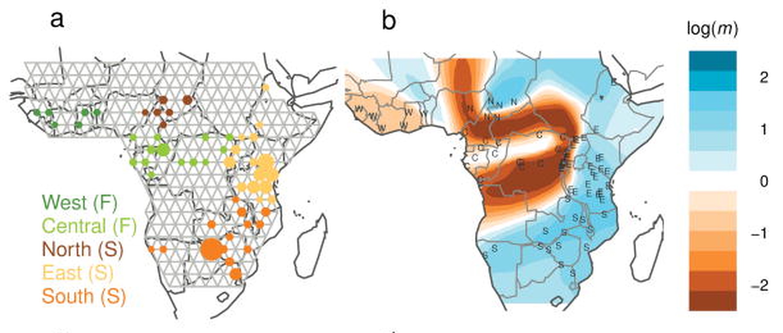
• IBD assumes anisotropy, and averages across the entire species/population
• Migration surfaces explicitly model gene flow among a connected grid of subpopulations, and can highlight areas of reduced or increased gene flow.

Isolation by Distance is a nonspecific pattern, and most formulations and models assume anisotropy, i.e. equal patterns at all places and in all directions. This assumption of anisotropy is patently false in nearly all species of any evolutionary interest: for example, the rate of migration in terrestrial species between Italy and the Balkan Peninsula is likely to be lower than would be expected due to the great-circle distance due to the intervening Adriatic Sea. Ideally, we would like to know the historical patterns of gene flow across the landscape in a way that allows for the complex and heterogeneous networks of historical gene flow observed in natural systems. These desires led to the development of a series of methods that model migration explicitly among the interconnected landscape of subpopulations, most notably EEMS.

Reading List

• Petkova et al., “Visualizing spatial population structure with estimated effective migration surfaces”, Nature Genetics (2015)

Isolation by Environment

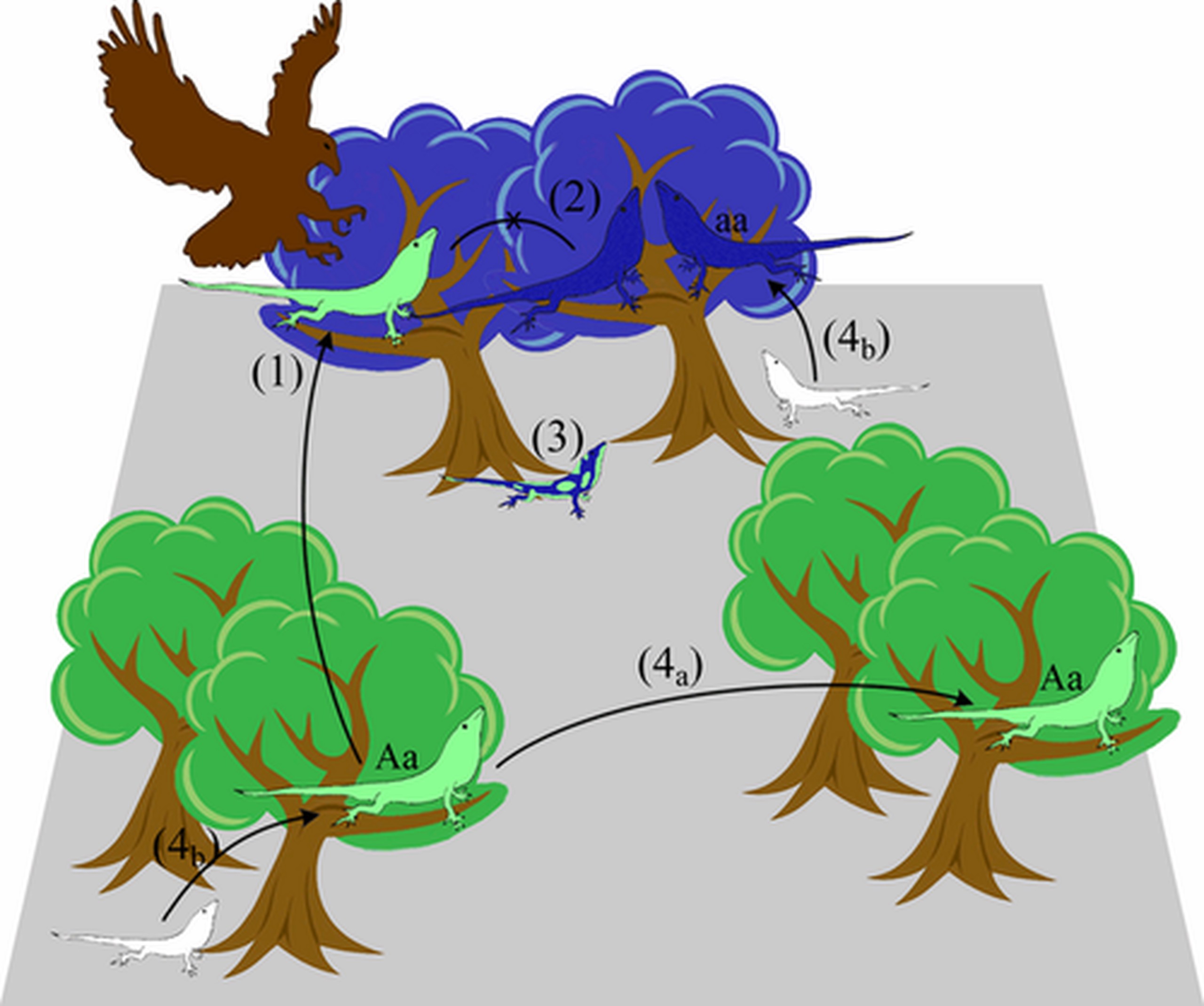
• Isolation by Environment: populations occupying similar environments are more closely related than would be expected simply by IBD (i.e. $G \sim E | D$)

So far, we have not considered the natural environment as a force shaping the spatial genetic structure of populations. Isolation by Environment describes a pattern in which individuals that share similar environments are more genetically similar than individuals from differing environments, after accounting for their geographic proximity (IBD). IBE has many forms: Local adaptation can lead to spatially-structured populations exhibit isolation by environment (at least at adaptive loci). Additionally, numerous non-adaptive processes can generate a pattern of IBE, for example synchronous flowering due to temporal patterns of rainfall.

Reading List

• Wang & Bradburd, “Isolation by Environment”, Molecular Ecology (2014)

Genome-average vs local

• Rest of talk will zoom from genome-wide average methods to methods considering genome windows and then individual SNPs.

Until now, we have considered genomes to be monolithic units uniformly experiencing spatial genetic differentiation. We know that the various loci comprising an individual’s genome exhibit different evolutionary trajectories, including where spatial genetic structure is concerned. Specifically, the above methods and models average the heterogeneous signal across assayed loci. Below, we will consider methods that treat each locus individually, and allow us to inspect how geography and the environment have affected loci specifically.

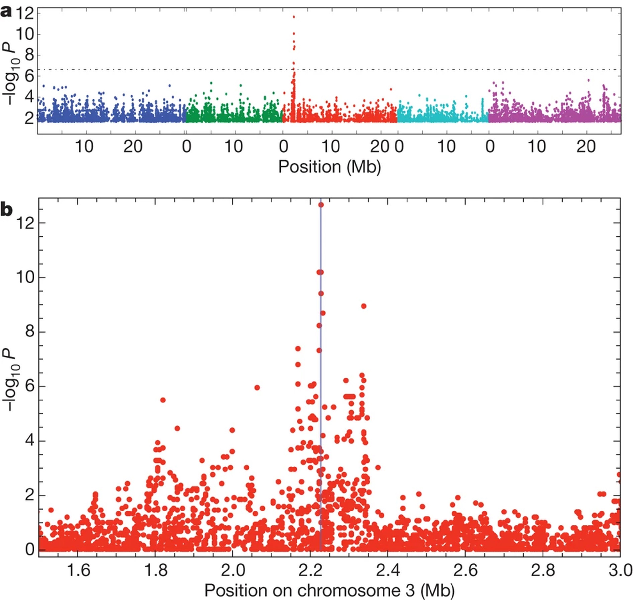
An aside: GWAS primer

• GWAS: statistically associate variation in trait with variation at each SNP in some experimental population.
• “Hypothesis generation”: find that variation in SNP x is statistically linked to trait Y

Before we discuss Genotype-Environment association, we should briefly cover Genome Wide Association Studies (GWAS), on whose logic GEA is based. GWAS is a statistical technique that links variation in one or more traits to genetic variation within a population. Natural populations are sub-sampled to form balanced core sets (e.g. RegMap; 1kg), and traits are measured on individuals of each genotype, typically in a controlled experiment. Then, at each identified SNP within the population of interest, we associate trait variation to genetic variation, controlling for background genetic variation (e.g. Population Structure). Typically, GWAS models are fit as a LMM with fixed SNP effects and covariates, and a random effect that controls for population structure: $\mathbf{Y} = \mathbf{W}\beta + \mathbf{G_s}\gamma + \mathbf{g} + \mathbf{\epsilon}$; $\mathbf{g} \sim N(\mathbf{0}, \sigma^2_g\mathbf{K})$, where $\mathbf{W}$ is a matrix of covariates, $\mathbf{G_s}$ is a vector of SNP genotypes, and $\mathbf{K}$ is a realised kinship matrix describing samples’ shared ancestry. In reality, GWAS are often performed using accelerated or heuristic forms of this full model, but results will be approximately equal.

Genotype-Environment Associations (GEA)

• NB: not to be confused with Gene-Environment interactions (GxE) within functional studies.
• Essentially a GWAS, but where our “trait” is a specific environmental variable, or a multivariate representation of the environment.
• Very many statistical methods, generally less well-polished than traditional GWAS.
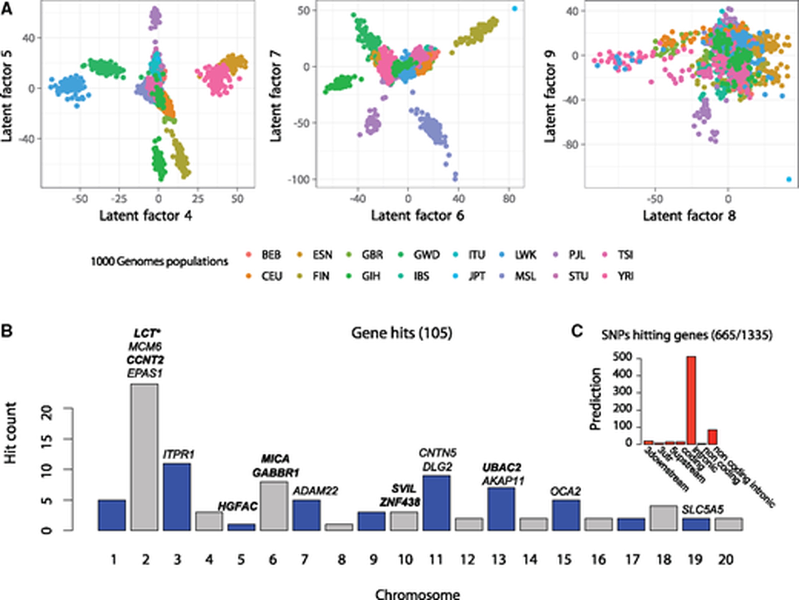
• LFMM and RDA are the leading modern approaches

In GWAS, we associate variation in some trait with genetic variation to form hypotheses regarding the genetic basis of this association. GEA extends this logic to form hypotheses regarding the genetic basis for adaptation to a specific environment or along some environmental cline. GEA is a particularly useful method of generating molecular hypotheses regarding environmental adaptation, as it operates a “level above” traits, and therefore will find association where either an unknown trait or multiple traits underly environmental adaptation. However this generality comes at a cost: GEA are more statistical challenging, and their design is susceptible to many more foibles than the design of a GWAS experiments. In particular, one must be very diligent to control not only for population structure a la GWAS, but also for spatial autocorrelation in the environment between sampled localities (in particular see Lotterhos and Whitlock’s 2015 paper below).

Like GWAS, GEA is a general method, and can be implemented in a diverse set of models and tools. The two leading approaches are Latent-factor Mixed Models (LFMM), and Redundancy Analysis (RDA). LFMM models have a similar form to GWAS, however instead of having random effects derived from an empirical kinship matrix, the random effect in an LFMM model accounts for $k$ Latent factors which are a lower-rank representation of the broad-scale structure in the dependent variable. While not strictly true, I consider this similar to accounting for the $k$ leading eigenvectors (“PCA axes”) of the similarity matrix of the dependent variable. While this is not guaranteed, the hope is that these latent factors will cover all sources of confounding, including spatial autocorrelation and kinship/population structure. RDA is a quite different multivariate statistical framework, in which variation in response variable(s) is explained by variation in predictor variable(s). RDA has the advantage of more flexible multivariate associations, at the cost of a less robust approach to determine the significance of individual SNPs (significance is typically reported as a Z-score of association to the underlying redundant axes). LFMM is a more general-purpose association toolkit, can handle multivariate environments, can perform regularised regressions, and has a more robust approach to determine statistical significance of each SNP locus.

Methods

• LFMM: implemented in a series of R packages (LEA, lfmm). Be sure to use the more recent lfmm2 implementation, which uses ML inference instead of the older version that uses MCMC.
• RDA: implemented in the vegan R package, see Brenna Forester’s paper and tutorials below.

Reading List

• Forester, “Detecting multilocus adaptation using Redundancy Analysis (tutorial)”
• Forester, “Comparing methods for detecting multilocus adaptation with multivariate genotype-environment associations”, Molecular Ecology, 2018
• Caye et al., “LFMM 2: Fast and Accurate Inference of Gene-Environment Associations in Genome-Wide Studies”, Molecular Biology and Evolution, 2019
• Lotterhos and Whitlock, “The relative power of genome scans to detect local adaptation depends on sampling design and statistical method”, Molecular Ecology, 2015
• Hoban et al., “Finding the Genomic Basis of Local Adaptation: Pitfalls, Practical Solutions, and Future Directions”, Am. Nat, 2016

About this tutorial

Text by Dr. Kevin Murray, Weigel Group, MPIDB, Tübingen, DE.

Most images looted from their original papers as cited/credited.